TRUE FILM EMULATION: Building a Photochemical Pipeline
- ARC Brand & Creative

- Mar 20
- 9 min read

Film emulation covers a lot of ground. LUT packs, PowerGrades, process-based plugins. They all aim for the same goal but get there differently, and the differences matter more than most people realize. We've tried most of them, and have always yearned for something better...something more realistic to the nature of process of film. We developed a film emulation plugin is a process-based photochemical pipeline built from measured sensitometric scan data of the Kodak Vision3 250D negative and Kodak 2383 print stock combination. It models what film does rather than approximating what film looks like.
Before / After


We’re not the first to take this approach, and we want to be upfront about where we sit in the landscape. FilmBox by Video Village set the bar for process-based film emulation. Genesis by Procolorist, developed alongside a two-time Oscar-winning Kodak film chemist, approaches the problem from the chemistry itself. Based on what both teams have shared publicly, they appear to have access to independent negative and print curve datasets that allow each stage to be modeled discretely. That’s a level of data granularity we don’t have.
Our data captures the combined result of 250D developed and printed through 2383. We’re working from the final output of the neg+print system, not from independent curves for each stage. That distinction shapes both the strengths and the honest limitations of what we’ve built.
LUTs, PowerGrades, and the Order of Operations
A well-built 3D LUT from real sensitometric data can be remarkably accurate. Tone curves, cross- channel coupling, saturation behavior at every exposure level, all encoded faithfully. The format gets a bad reputation from poorly built packs, but that’s a problem with execution, not with LUTs. Where a single combined LUT stops is decomposability and spatial processing. The entire neg-to-print chain is baked into one mapping. You can’t adjust the negative separately from the print, change the printer lights without regenerating the table, or model anything that depends on neighboring pixels.

Splitting the LUT into separate negative and print transforms is a genuine improvement. With a matched neg LUT feeding a print LUT, you can place grain and halation between them and get convincing results. The grain sits in the negative’s density domain, the halation operates on the negative’s output, and the print LUT responds to both. But there’s a deeper issue. Halation physically happens at the CMY exposure level, after the spectral
sensitivity matrix sorts light into layers but before the H&D curves develop that exposure into density. The halation-modified exposures then flow through the curves, so the film’s nonlinear response shapes the scatter naturally. With a neg LUT, the H&D curves are baked inside. You can’t insert halation before them because that intermediate stage doesn’t exist as an accessible signal.
Grain has the same structural problem. It occurs at the individual CMY dye layer level, before the dye
absorption matrix combines layers into composite density. That cross-layer contamination through
the DAM gives film grain its color character. With a LUT, the DAM is baked in. Grain can only be
added to the composite output, not to the individual layers that feed into it.
The architectural argument for process-based emulation comes down to this: spatial processing
requires access to specific intermediate stages that don’t exist in a LUT-based workflow, even a well-
designed split one.
PowerGrades offer an interesting middle ground. Discrete Resolve nodes can theoretically place
spatial operations at any point in the chain. The limitation is data fidelity: a curves tool has finite handles and a color warper has finite control points. A well-built LUT can capture more measured
data than a PowerGrade can express. You gain the correct order of operations but lose precision at
each stage.
System Modeling vs Camera Profiling
There’s a different approach to film emulation that doesn’t model the film chemistry at all. Camera
profiling shoots a known test chart on both a digital camera and real film, processes and scans the
negative, then builds a transform that maps the digital camera’s output to match the scan. The result
makes Camera X look like it was shot on Stock Y and scanned at Lab Z. Most commercial film emulations work this way, whether they say so or not.

The approach has real strengths. It captures the entire analog chain empirically: the scanner’s response, the lab’s chemical conditions, the interaction between the sensor’s spectral sensitivity and the stock’s. Serious profiling workflows shoot multiple exposure brackets and build transforms across a wide dynamic range. If the goal is to match a specific camera to a specific scan of a specific stock, profiling gets there efficiently because it absorbed all those variables at once.
The two approaches aren’t mutually exclusive. You could use profiling data to calibrate the input stage of a system model, building a better spectral sensitivity match for a specific sensor while still running the full photochemical pipeline underneath.

But each answers a different question. A profiled transform is built from a specific camera’s color science. Shoot on a different camera and the profile needs to be rebuilt, or you need per-camera IDTs that normalize to a common working space first. A system model works from scene-referred data in a defined color space. Any camera that delivers proper ACEScct gets the same film behavior without camera-specific calibration.
Then there’s the spatial dimension. Grain, halation, acutance, emulsion MTF. None of these exist in a profile. They’d need to be added separately, operating on the final output rather than at the intermediate stages where they physically occur.
The honest gap in system modeling is the subtle color character of the full analog chain. A real negative on a real scanner has a quality that’s the sum of dozens of small variables: gelatin spectral absorption, the optical path of the scanning element, minor chemical inconsistencies. A system model doesn’t individually capture these.

But those variables change from scan to scan. No two passes through the same stock at the same lab look identical. Matching one specific scan with scientific precision isn’t more accurate to film. It’s more accurate to one particular instance of film. When a colorist says footage looks like film, they’re responding to contrast roll-off, color crossover, grain that lives in the image, halation softness, the way saturation tracks with luminance. Those are system-level behaviors. That’s what system modeling captures.
What a Photochemical Pipeline Models
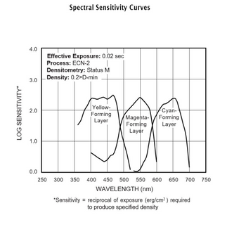
When light hits motion picture negative, it passes through multiple emulsion layers, each sensitive to
a different part of the spectrum. The sensitivity isn’t perfectly isolated. There’s measurable cross-talk
between layers. That spectral sensitivity matrix is one of the first things you model.
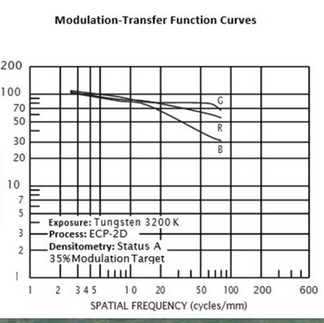
Each layer has its own nonlinear density response: the H&D characteristic curve. Each channel has its own gamma, shoulder, and toe. Then there are interimage effects between layers, dye absorption characteristics, and the grain structure of the emulsion. Our plugin models each of these from measured Kodak data.


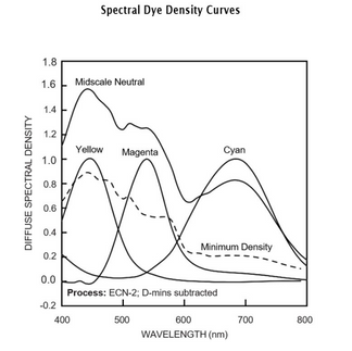

(Source: Kodak Technical Publication H-1-5207)
Every Stage Has a Correct Domain
The biggest improvement in our architecture came from something that sounds obvious: each stage
of the photochemical process happens in a specific physical domain, and doing the math in the wrong domain compounds errors through everything downstream.
Exposure is linear. Density is logarithmic. Dye coupling is multiplicative in transmittance, additive in log space. Do a log operation in linear and the math is wrong. Not approximately wrong. Wrong. Our earlier architecture did everything in one domain and compensated with correction layers. Each one was patching artifacts from upstream operations in the wrong space. We restructured so ever operation lives in the domain where it physically occurs. Exposure scaling in linear. Characteristic curves on log-exposure values. Dye absorption in density. Each domain transition is explicit and exact.
The Unified Pipeline

Our earlier build used separate plugins for the negative and print stages. The negative produced compound Status M density, then converted back to scene-referred encoding for output, because that’s how the host passes data between plugins. The print plugin received this signal, decoded it, and tried to reconstruct the density it needed.
That reconstruction was lossy. Compound Status M density has specific cross-channel relationships from the dye absorption matrix. Converting to scene-referred linear and reconstructing on the other side doesn’t recover them. The result was gamut clipping, midtone color shifts, and highlight behavior that never matched the data.
The fix was to stop splitting. After the dye absorption matrix produces compound density, it flows directly to the print curves. No conversion, no reconstruction, no round-trip. Every compensation stage became unnecessary. The print’s color character emerged cleanly from the data.
Defined Input, Defined Output
Our plugin operates as a Look Modification Transform within the ACES pipeline. It receives ACEScct, processes through the full neg+print photochemical chain, and outputs ACEScct. It is not a display transform. The output is scene-referred data shaped by the film’s response characteristics, and it still needs an Output Display Transform to reach your monitor.
The film look lives upstream of display. You can change your ODT for different deliverables without touching the grade. The same film-processed image goes to Rec.709, P3, or HDR through whatever output transform is appropriate.


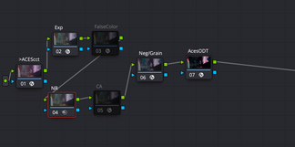

ACES pipeline
The Print Stock
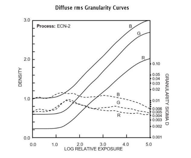
The negative is half the story. Kodak 2383 has specific cross-channel coupling between its cyan, magenta, and yellow dye layers, and that coupling is what gives a projected print its color quality. We model this from the full sensitometric dataset: not just the 19 neutral patches used for per-channel density transfer, but 1,729 measured patches including saturated colors that reveal how the print responds to narrowband colored light versus broadband white.
With the pipeline running cleanly from measured data, the print stage becomes a real creative surface. Printer lights add per-channel density offsets before the print curves, exactly as an additive printer does. Because these offsets feed through the print stock’s nonlinear response, the result has the natural compression of a real print adjustment, not a digital gain change.
Independent highlight and shadow contrast controls, combined with split temperature and tint, let you establish a complete print setup: a specific combination of contrast and color that defines the visual identity of a project. What you feed the plugin is your on-set intent. The negative models how the stock responds to that light. The print setup is the lab’s interpretation of how this story should feel on screen.


(Source: Kodak Technical Publication H-1-2383)
Grain, Halation, and the Spatial Problem
Film grain isn’t noise. It’s the statistical result of silver halide crystals activating during development,
and it depends on the density underneath it, the film format, and the spatial relationships between
crystals.
Our grain engine uses calibrated crystal counts for the specific stock. The sigma at each pixel comes from per-layer dye density: zero grain at unexposed film, maximum at mid-density, decreasing at full exposure where all crystals are already activated. It’s applied additively in the density domain at the individual dye layer level, before the absorption matrix combines layers. That’s where grain physically happens in real film. The grain propagates through the dye absorption cross-contamination, and the print stock responds to it naturally. The 2383’s curves compress grain in the shadows and highlights while accentuating midtones, which is what happens in projection. Spatial correlation uses neighborhood sampling for clumping, and grain scales with both film format and timeline resolution.

Getting grain to feel truly embedded requires more than placing it at the right pipeline stage. In real film, the grain crystals are the image. There is no detail finer than the grain structure. We model the emulsion’s modulation transfer function as a pre-soften that couples image resolution to grain resolution. Acutance, the edge enhancement from developer diffusion, then restores the edge contrast that makes film feel sharp despite the grain. MTF and acutance work together so the grain doesn’t sit on top of the image but is woven into it, the way it is in a real emulsion. All spatial effects scale with both film format and timeline resolution, so the same physical behavior looks correct from 1080p to 8K.
Grain Comparison:


Halation is caused by light passing through the emulsion, hitting the film base, reflecting off the anti-halation backing, and re-exposing the emulsion from behind. Most implementations apply this to the final RGB image. We apply it to the per-layer CMY exposures after the spectral sensitivity matrix,
before the characteristic curves develop density, which is where it physically occurs.

The cyan layer sits closest to the base and gets the most scatter. Magenta gets moderate scatter. Yellow gets the least. A bright blue source produces almost no halation; a bright red source produces strong scatter. Per-layer thresholds get that right where luminance-based thresholds can’t. Because this operates in the unified pipeline, the halation-modified exposures flow through the H&D curve and the print stock responds to them naturally.
Before/After 16mm:


The Question of Data

Tools like FilmBox and Genesis seem to have access to independent curve data for each stage,
modeled from discrete measurements. Our data captures the combined output: a combined scan of
the 250D negative developed and printed through 2383. We’ve decomposed that result into constituent stages using the physics of the system. The results are accurate to the measured data, but the decomposition involves modeling assumptions that independent curve data would not require. A balanced, properly exposed image run through our pipeline comes out with the authentic tonal response, color coupling, grain structure, and spatial characteristics of the 250D+2383 combination.
The inherent color signature is there. At default settings you get a neutral representation of what that
stock combination looks like. The print controls let you build from there.

Is full curve separation strictly necessary for a tool that produces a filmic image a colorist can work with? There’s a reasonable argument that it isn’t. Real film scanning introduces its own artifacts, its own interpretive layer. A precise emulation of the measured combined system, with real creative tools in the print domain, may be more useful than a more physically complete model that reproduces the imperfections of a particular scanner or lab setup. We’re not claiming our approach is better. We’re saying it’s a valid path, and the results support that.
What’s Next?
The unified architecture was the turning point. The pipeline runs as a single GPU plugin: negative,
halation, emulsion MTF, grain, acutance, and print stock in one node. We’re still finding things in the data, and each improvement compounds on the ones before it. More technical breakdowns and workflow guides are coming.


Comments